Dynamics
Dynamics and Kalman filters
These mathematical models, use Newton's laws and Euler's equation for rigid body motion, to iteratively and accurately simulate the physics of various rotating objects. The the models were created in order to prove the implementation of the linear and rotational dynamics for Kalman filtering on the guidance computer of the Medway Makers autonomous aircraft project. The prototype microcontroller and sensor board appears at the bottom of the page.
Because the models are written in Java-script, running in real-time, simultaneously these iterative mathematical models' accuracy is limited by available computing power.
To see a model at its best, click on it to run it by its self and full screen, allowing more precision. Then by resizing the screen you can see all the physical perameters for the object, but you will need to refresh after doing a resize!
Rotating tape
I chose a number of physical situations to model that I could see video for, or could reproduce at home.
Astronaut Chris Hadfield kindly helped by letting go of a roll of duck-tape in zero gravity in the International Space Station to verify that my mathematical model could reproduce it's spinning motion. It would be closer if I spent longer getting the initial conditions dead right.
Cycle Wheel Precession
Take a bicycle wheel and hang it by one side of the axle from the ceiling on a string. Release it and it swings like a pendulum but spin it and it will remain vertical and wobble and precess its way around.
The model is only an approximation in so far as in the model the wheel is hung from the centre of the axel with a rotational torque being applied to match that that is applied by the offside string in reality. Also all the mass of the wheel, in the model, is in the outer rim. I was very pleased to see both the precession and wobble matched in the reality and my model.
No Rotation
Without rotation the wheel simply swings like a pendulum. The real wheel looses energy as the axel rotates and also some energy is converted to actual swinging on the string.
Rotation
With rotation the wheel precesses with a slight wobble.
The phenomena is accurately modelled here.
All these simulations use Euler's equation for rotating rigid bodies.
Intermediate Axis Theorem
Most spinning objects have three main axes of rotation with the exception of things which have rotational symmetries like spheres and cylinders.
Rotation about the axis with minimum moment of inertia or maximum moment of inertia are inherently stable, however the axis of rotation with intermediate moment of inertia is inherently unstable.
If we spin an object slightly off axis on each of the three axes,
the spinning on the intermediate axis will perform an odd flip where as the other axes will spin in a stable manner.
The previous video of the "Dancing T-handle" shows this "intermediate axis" instability, but any object spun on its intermediate axis will show the same instability as the T-handle does.
Try it with your mobile phone, most mobile phones are perfect for seeing this happen in real life. It doesn't work though if two of the moments of inertia are equal, most are not.
The next three frames model the same object, a mobile phone perhaps, spinning on its three axes. The angular momentum is set to 2 radians per second on the main axis of spin in all the frames, but with 0.02 radians per second spin on one of the other axes just to show up the instabilities.
As an addendum I had to put up a further frame where the spin is again about the intermediate axis but the 0.02 radians per second spin has been reduced further to only 0.0002 radians per second.
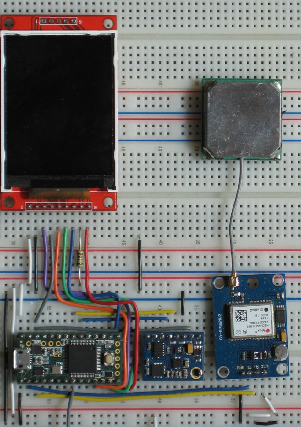
Guidance Computer Prototype
A picture of the prototype guidance computer appears in the following frame.
The code for the guidance computer will be written in 'C' and will learn from the Java-script presented here.
There will be considerable hardening of the code. In any critical software there will be no use of the heap, the code will use pre-allocated or stack based memory only. All neumeric and other exceptions need to be caught and handled properly.
The image shows a screen on the top left. The silver square on the right is the GPS aerial and below that the GPS receiver. To the left of that is the accelerometer/magnetometer board. On the bottom left is the microcontroller on which the guidance software will run.
Kalman Filter
The next image simulates a craft in the real world in retain the desired position and orientation using its (simulated) onboard guidance computer and sensors, GPS, magnetometer and linear and angular accelerometers. These provide noisy inputs to the guidance computer which uses Kalman filters to improve the result.
- Grey shows the position according to the sensors with noise
- Yellow shows the position calculated by the the guidance computer using the equations of motion.
- Green shows the position according to the guidance computer after combining the calculated and sensor information using Kalman filtering, and lastly
- Red shows the position in the simulated real world.
Controls
You can move the grey spot target position by placing the mouse on the image and then moving the scroll wheel slightly. Rolling the scroll wheel moves the spot in the third dimension away or towards you.
You can change the target orientation of the craft by holding down the left mouse button and moving the mouse or rolling the scroll wheel. You may need to refresh the page to stop the scroll wheel scrolling the whole page!
The implementation is an extended Kalman filter. The Kalman gain matrix is shown in the background. Elements very close to 0 are shown in a darker colour. It is broken up into blocks of 3x3 relating to the components of the vectors.
Columns relate to position, rotation, angular velocity and linear acceleration 3d vectors.
Rows relate to position, rotation, linear velocity, angular velocity, force and torque 3d vectors.